Characterizing the material properties of polymers for automotive applications

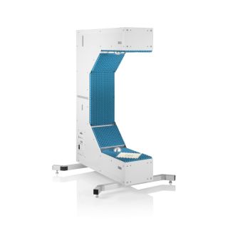
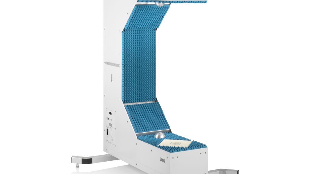
Automotive radar sensors can be well hidden behind bumpers, but require to be transmissible in the respective frequency domain. To effectively hide the sensors, the radar-transparent areas are usually required to have the exact same shade of color as the rest of the vehicle. To select proper colors and coatings for such bumpers, the respective material properties must be known. In the past, either quasioptical or waveguide based setups, both using vector network analyzers (VNA), have been used. This application card demonstrates a simplified method for material characterization in the automotive radar frequency domain (76 GHz to 81 GHz) based on the R&S®QAR50 automotive radome tester.

R&S®QAR50 automotive radome tester

Your task

Automotive bumpers are typically made of several layers: The structural base material (typically being a PP or PC compound) gives the bumper its actual form and is the thickest layer. However, it is not necessarily the layer with the greatest influence on the radar signal, as it can generally be well adapted. Using different fillers, the properties of the base material can be adjusted to achieve a better UV resistance, rigidity, radar attenuation, etc.

A primer is applied as a second layer and to help the actual color adhere to the base material. The thickness of the primer is typically within a couple of micrometers.

Therefore, a slight measurement uncertainty is required for measuring the thickness of this and all subsequent layers.

The third layer is the actual color applied to the primer. The thickness of the color layer depends, among other factors, on the opacity of the used paint and is very thin.

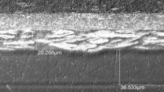
To protect the color from environmental influences, a clear coat is typically applied as a fourth and top layer. To estimate the electromagnetic properties of all layers, their thickness needs to be known as precisely as possible. For the example used here, a scanning electron microscope was used to determine the thickness of each layer (see figure below).

Fig. 1: Micrograph showing the different layers of an automotive bumper sample: base material (PP), primer, paint, clear coat (top to bottom).
Open Lightbox

All layers must be characterized independently. There are different ways to do so. This application card is based on four different samples to characterize all four layers:

  • In the first step, only the base material is analyzed
  • The second step is then analyzing the primer on the previously characterized base material
  • The third and fourth step follow the same logic

To create such a micrograph, the sample has to be destroyed. Therefore, all measurements described above need to be taken beforehand. The following section covers the required RF analysis of the samples.

Rohde & Schwarz solution

Permittivity estimation with the R&S®QAR50

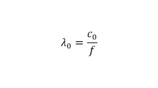
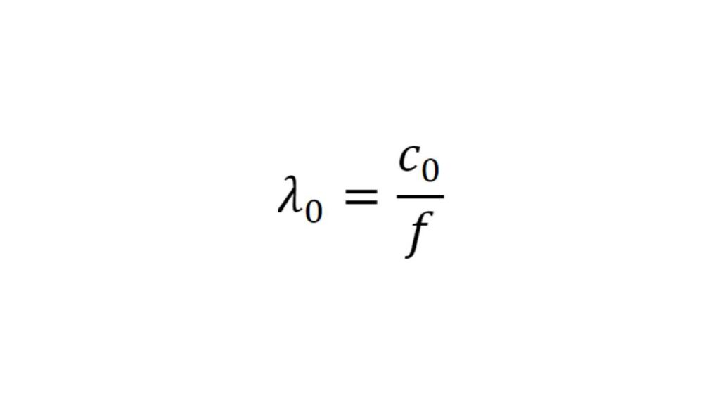
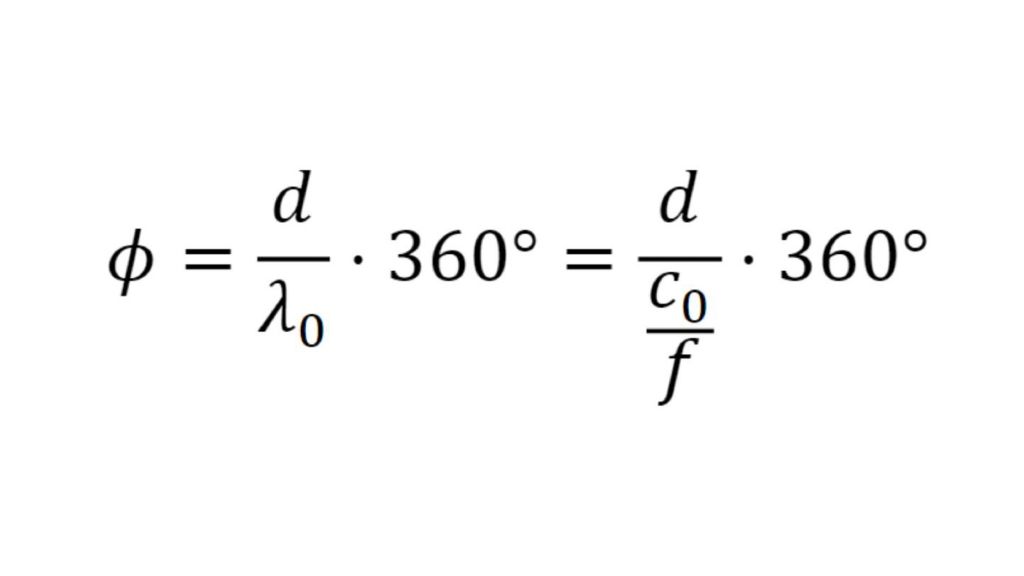
The permittivity of the sample influences the speed of the electromagnetic wave inside the material and slows down its propagation. Reducing the speed of the electromagnetic wave reduces the wavelength inside the material. With frequency f and speed of light c0 in a vacuum, the wavelength λ0 is defined as:

Formel 1

Typical automotive radar frequency: fradar = 76.5 GHz, wavelength: λ0 = 3.92 mm.

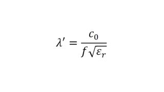
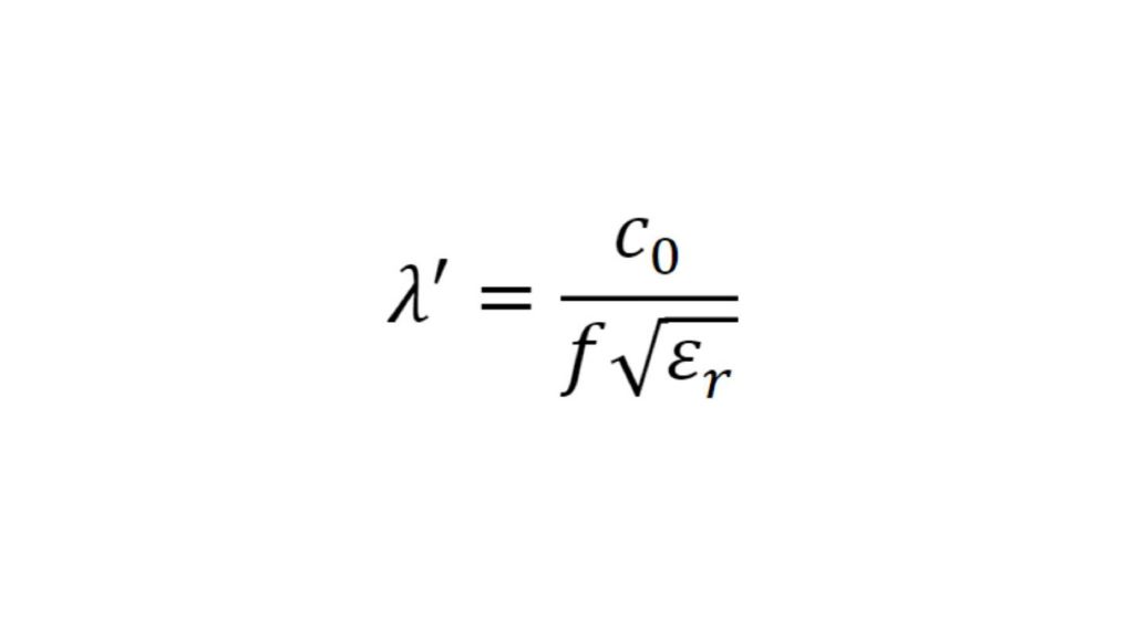
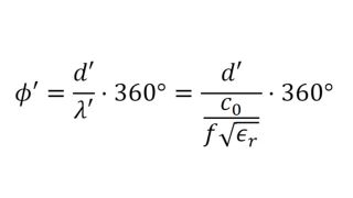
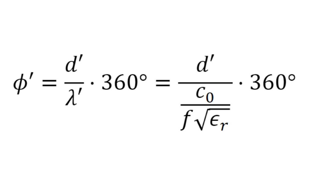
The wavelength inside a given material with the relative permittivity εr is calculated as:

Formel 2

Taking the sample polypropylene (PP) sheet with εr ~ 2.5, the wavelength in the PP sheet is calculated as λPP = 2.34 mm. Since the permittivity reduces the wavelength, it can be calculated using the measured phase if the thickness of the material under test (MUT) is known.The general procedure is demonstrated below.

Calculating the permittivity using relative phase differences

The R&S®QAR50 is normalized to air propagation and every material positioned between the two clusters alters the phase at the receiving antennas. To characterize the sample, we are now interested in the phase difference caused by the sheer presence of the MUT within the measurement path.

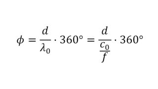
For reference, the phase Φ in degrees over distance d in free space is calculated as:

Formel 3

The phase Φ’ through material of thickness d’ is calculated as:

Formel 4

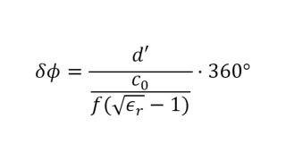
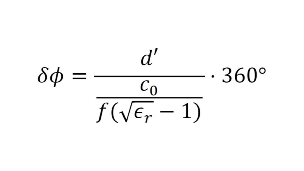
Therefore, the phase δΦ change as seen by the R&S®QAR50 is the difference between Φ and Φ’ above and thus corresponds to:

Formel 5

For the example above using a 2.92 mm PVC sheet with an estimated permittivity εr ~ 2.5, this leads to an expected phase difference of δΦ ~ 158°.

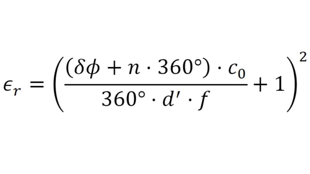
As we are measuring the phase difference δΦ using the R&S®QAR50 and want to calculate the permittivity εr , the above formula must be rearranged slightly to:

Formel 6

The resulting permittivity is not unique, as the phase difference could unknowingly be multiples of 360°. For n Σ N0 all possible solutions can be calculated.

For multilayer samples, all layers except the one to be determined need to be characterized already. Only then can the known layers be normalized out.

To simplify the above-described calculations, a software is available for the R&S®QAR50. The permittivity calculator, which utilizes the R&S®QAR50 precise phase measurement results, is introduced below based on an example.

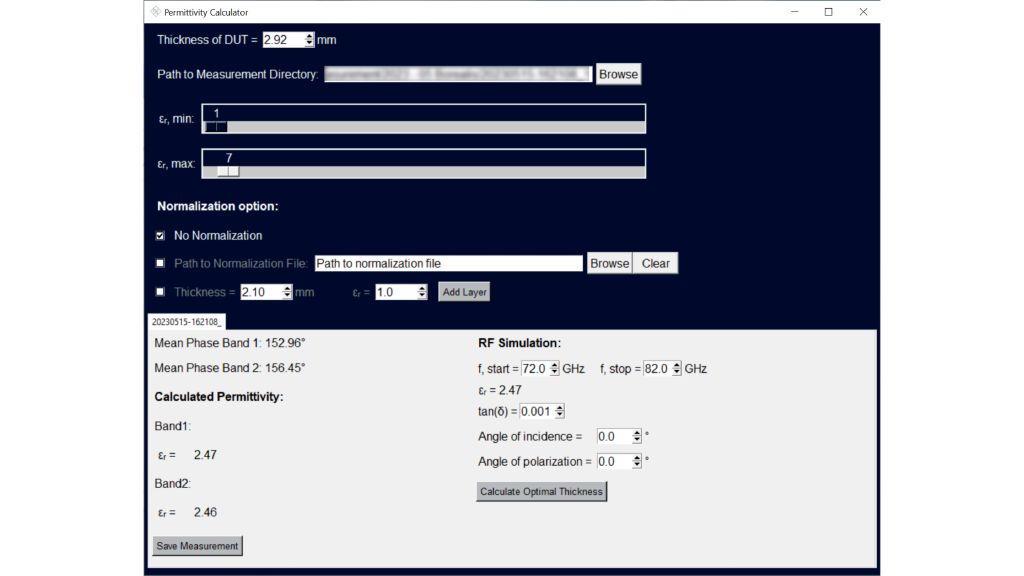
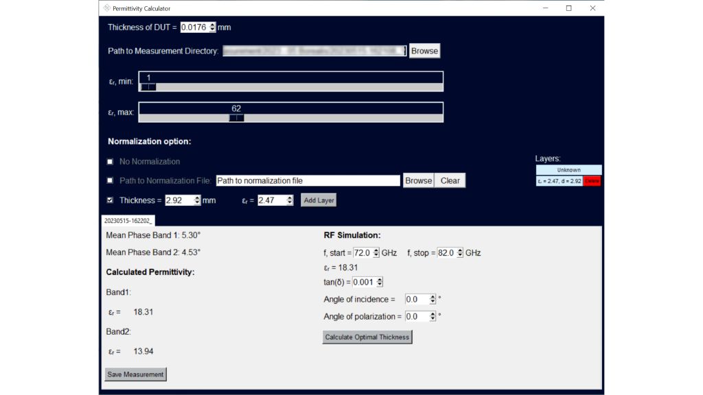
Fig. 2: The base layer is loaded into the permittivity calculator. The calculated permittivity due to the phase change of 153° at 76.5 GHz is εr = 2.47.
Open Lightbox

Exemplary characterization of a painted bumper sample

Using the same exemplary set of samples as in the previous paragraphs, the thickness of the different layers is known and plates with individual layers are available for characterization. For the thickness of the individual layers, see Fig. 2.

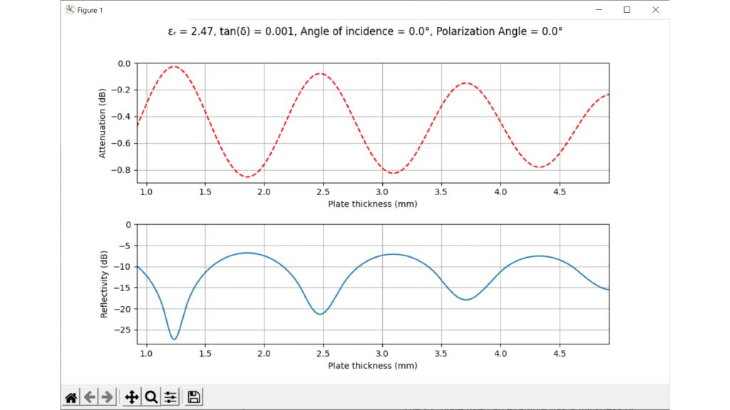
Fig. 3: Optimal thickness of our characterized PP sheet with calculated permittivity of εr = 2.47
Open Lightbox

The base PP plate has a thickness of 2.92 mm and causes a measured phase difference of ~ 153° at 76.5 GHz. Using the measurement results as input parameters, the tool calculates an εr = 2.47 for that specific plate. Fig. 2 shows the result of the calculation in the software.

If in an application this material is used as a single-layer radome, it would be interesting to know what the optimal

thickness in terms of radar transparency would be. To provide a quick and easy solution, the permittivity calculator

has an optimal thickness calculation tool as shown in Fig. 3.

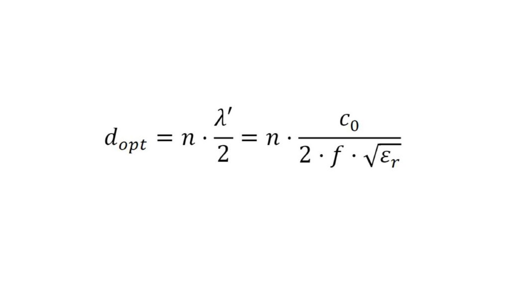
Using this tool, the optimal thickness dopt can be derived from the minima in reflection and transmission loss. Those reflection minima are correlated to the resonance frequency of the sample and occur at multiples of half the wavelength within the material.

Formel 7
Fig. 4: Adding normalization layers to characterize the primer, color coat and clear coat

To characterize the remaining layers, the base material needs to be normalized out. Since the permittivity of the material is now known, this can be done for the next plate containing the primer.

Therefore, a normalization layer is added in the software and the next measurement result is loaded.

The normalization can either happen on a previous measurement or by manually adding a layer with a defined thickness and permittivity. In our example, the normalization layer with thickness 2.92 mm and εr = 2.47 is manually added and visualized on the right side of the tool. Based on the measured thickness of the primer (see e.g. Fig. 1) and the measured phase shift of 5.3° using the R&S®QAR50, the calculation comes up with an estimated permittivity for the primer of εr = 18.3. The corresponding result is shown in Fig. 4.

As soon as the second layer is characterized, the estimation of the remaining layers can be performed according to the steps described above. The already characterized layers are added for normalization and the unknown permittivity is calculated by the tool.

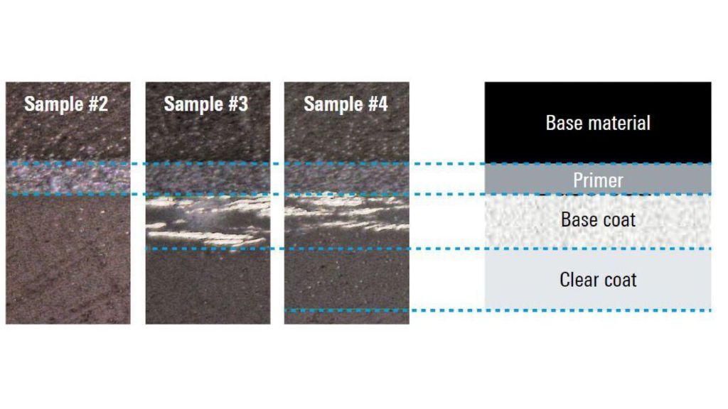
Since the thicknesses of the layers across the samples might differ, care has to be taken when adding normalization layers. Fig. 5 shows the micrograph of the used samples as seen using an optical microscope. Significant differences in thickness of the color layer can be spotted for the intermediate sample #3 (used to characterize the color itself) and sample #4 (used to characterize the clear coat applied to the color).

Fig. 5: Micrograph of the three processed samples showing significant differences in thickness of some layers. Sample #1 (raw PP material) is not shown due to the different scaling.
Open Lightbox

A more detailed analysis of the topic together with a comprehensive comparison between the R&S®QAR50 and a vector network analyzer can be found in [1].

The permittivity calculator is available on request through the Rohde & Schwarz distribution channels.