
Your task
As a development or test engineer, you use an R&S®RTP, R&S®RTO or R&S®RTE oscilloscope in your daily work. You store recorded waveforms for archiving and documentation or for further processing that is beyond the oscilloscope’s functional or performance limits. Using the ASCII format (csv file suffix) to store waveforms can potentially exceed the storage capacity. This format also requires a significant amount of time to transfer and process. Moreover, some information is unavailable when using the ASCII format instead of the binary format.
Rohde & Schwarz solution
The Rohde & Schwarz lab and performance oscilloscopes (R&S®RTP, R&S®RTO, R&S®RTE) all share the same format for binary waveform storage. The high-performance auxiliary Python RTxReadBin package allows you to handle binary files and obtain all of the necessary details for your documentation.
Application
In order to transfer the waveform from your instrument to your Python environment, you must prepare the Python IDE:
- Download the RTxReadBin package from the Rohde & Schwarz website
- Install the package on your system
- Acquire a waveform on your scope and store it as a binary file
Two files will be created: a waveform description file (*.bin) and a waveform data file (*.wfm.bin). The waveform data (loaded via the RTxReadBin function) may consist of the following:
- Analog channels
- Digital channels (MSO)
- Parallel buses (acquired via MSO)
- Analog channels (via ZVC)
- Math waveforms including spectra
- Tracks (automated measurement based waveforms)
For all of these signal sources, multiple acquisitions and multiple channels are supported if applicable.
After acquiring data with the Rohde & Schwarz oscilloscope, you can load it into your Python environment for further processing. For greater convenience, however, you can also leave the waveform where it is and enable network access to the data by mounting a CIFS share on your computer. Perform the following preparatory steps on the oscilloscope:
- Go to advanced sharing
- Select public profile and change the following parameters:
- Turn on network discovery
- Turn on file and printer sharing
- Turn on write access to public folders
Once you have completed these steps, you can connect to the scope using the following file path in your Python script:
r’\\<name of scope or IP address>\Users\Public\Documents\Rohde-Schwarz\RTx\RefWaveforms\<filename>.bin’
Be aware that because Python interprets the string, the \U character sequence will be interpreted and lead to an error. To avoid this, just add an “r” (for raw) in front of the string. You may be asked for credentials. Make sure you do not use authentication against the local Windows domain server. To do this, precede the local account instrument with a backslash:
account: \instrument
password: <your oscilloscope pw>
Alternatively, you can also download (drag and drop) the waveform from the scope using Windows Explorer.
Once these prerequisites are in place, you can load the module via the Python import and invoke RTxReadBin. The simplest way to do this is by providing the filename. The function returns three parameters: the vertical waveform data (y), the horizontal axis data (x) and the acquisition parameter (S).
> from RTxReadBin import RTxReadBin
> import numpy
> y, x, S = RTxReadBin(’<wfm filename>.bin’)
> y.shape
The vertical data (y) is a NumPy array with a shape of [<record Length>, <# of acquisitions>, <# of active channels>]. For an MSO waveform, the data type is just Boolean and for the parallel bus, it is an unsigned integer (uint16), bit-packed with the highest MSO index (MSB). For example, assume MSO lines D12, D7, D2 and D0 are connected and configured as a parallel bus. Then, the recorded data word will be stored as D12 ∙ 23 + D7 ∙ 22 + D2 ∙ 21 + D0 ∙ 20. For all other waveform data types, float32 is used. It is important to mention that the oscilloscope uses a different way of counting the history of acquisitions compared to Python. The oscilloscope starts with (1 - <# of acquisitions>) and counts up to 0 as the last acquisition. In Python, the counting is shifted and starts with 0 and ends with (<# of acquisitions> - 1) as the last acquisition.
The horizontal data (x) is a 64-bit float NumPy array with a shape of [<record length>]. If the data is stored in x/y interleaved format, the array is extended to cover all acquisitions [<record length>, <# of acquisitions>]. If a spectrum is stored, the x axis will contain the frequency axis of the spectrum.
The record length, number of acquisitions and channels can be easily retrieved by accessing the shape property of the return value y.
If not all of the parameters are required, they can be ignored using the standard Python techniques, e.g. by adding a list specifier (see example below) or using an underscore as a positional return parameter.
> y, x =
RTxReadBin(’<wfm filename>.bin’)[0,2]
There are two further (optional) parameters that can be specified in order to reduce the amount of allocated memory. The first parameter specifies the acquisitions of interest. The second parameter specifies the interval, time or frequency of interest. Both require a list with a length of two items. Be aware that the acquisition parameter follows the Python notation of a list. In the given example, two acquisitions (2,3) are returned.
> y, x, S = RTxReadBin(’<wfm filename>.bin’,
acquisitions = [2,4],
xInterval = [-2e-7,3e-7])
The remaining parameter S gives all of the details that are available in the header file. It is implemented as a Python dictionary. Not all of these parameters are important for the user. However, a few of them can be helpful for documentation and analysis. Since the waveform data in the y vector is just a float, the user cannot determine the original settings from this data. By examining the parameters in the header, however, the user can obtain the necessary information for documentation and postprocessing. For example, in order to understand the noise constraints for a measurement, it is important to have information about the settings for the vertical scale, offset, position and coupling.
Another example involves pulse repetition interval (PRI) analysis in radar applications. When one radar pulse per acquisition is captured using the segmented memory1), the list of timestamps from a segmented capture gives the trigger events over time, which are not available otherwise (S[’Timestamps’]). The time difference for consecutive trigger events provides the PRI sequence.
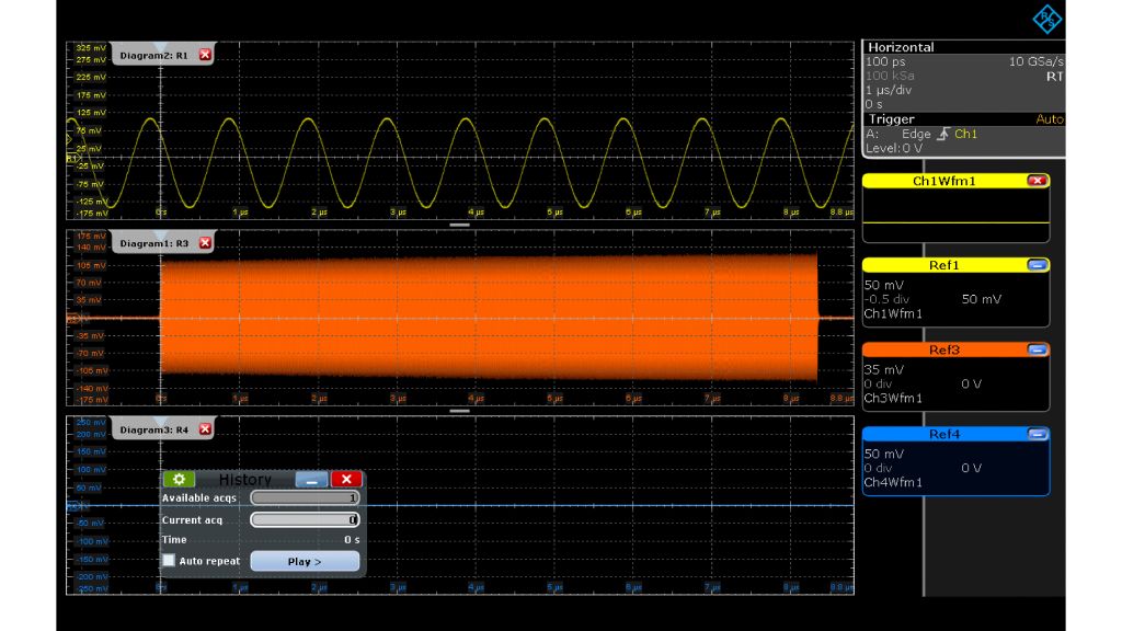
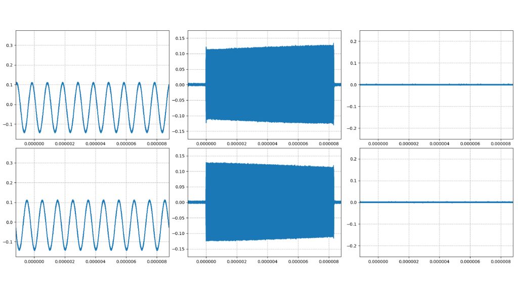
The next two plots show waveform data loaded on the scope and in a Python environment. Three signals are displayed:
- 1 MHz sinusoidal signal with offset
- Radar chirp alternating up/down
- Noise – no signal connected
The advantage of the RTxReadBin function is that it can handle waveform files with multiple acquisitions (history). When the same file is loaded, the oscilloscope only recognizes the last acquisition and displays an empty history.
1)See “Demodulating radar RF pulses with an oscilloscope” on the Rohde & Schwarz website:
Summary
The R&S®RTP, R&S®RTO and R&S®RTE are powerful oscilloscopes. The Python module (RTxReadBin) extends the instruments’ functionality by allowing you to access stored waveforms. For applications involving postprocessing, documentation or subsequent analysis procedures such as waveform comparisons, all of the waveform data is now available within a powerful Python environment.


